
Hello! Today we'll be going through some hands-on activities to help you get familiar with the steps involved in genome assembly and quality assessment.
The first thing you should do if you haven't done so is connect to the ConGen server. We'll be working exclusively in the RStudio browser interface that you should be familiar with by now, but if you have questions or problems at any point please feel free to ask! Just in case, here's a annotated picture of roughly what you should be seeing right now. If you are seeing something drastically different or something that you don't understand, let us know.
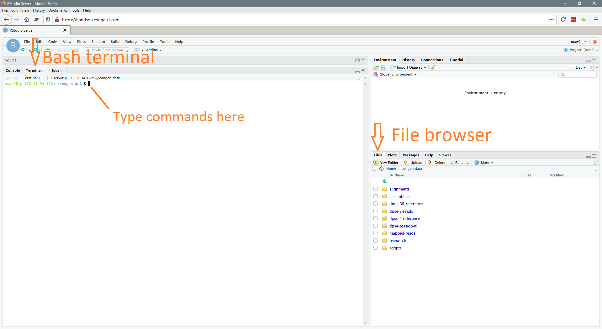
Most of our work will be done as bash commands typed in the Terminal provided by RStudio. Throughout this walkthrough, commands will be presented as follows:
this is an example commandFollowing each command will be a table that goes through and explains each part of the command explicitly:
| Command line parameter | Description |
|---|---|
| this | An example command |
| is | An example option used in the example command |
| an | An example option used in the example command |
| example | An example option used in the example command |
| command | An example option used in the example command |
The goal of providing these tables is to break-down some of the 'black box' that command line tools can sometimes feel like. Hopefully this is helpful. If not, feel free to skip over these tables when you see them!
A general convention among command-line software is to provide a help menu for programs that lists common options. These can generally
viewed from the command line with the -h option as follows:
<program> -h -or- <program> <sub-program> -hFor Linux commands, documentation is generally available with the man command (man is short for manual):
man <command>man opens a text viewer that can be navigated with the arrow keys and exited simply by typing q.
If you're ever stuck or want to know more about a program's options, try these!
Commands that you should run will have a green background. We will also provide some commands that are beneficial to see, but do not necessarily need to be run using a red background, like so:
this is an example command that won't be runAdditionally, one of the most important and often overlooked parts of bioinformatics analyses is to simply look at ones data. There will be several points where we stop to look at the output of a given program or command. When we do, a snippet of the output will be presented in the walkthrough as follows:
Here is some made up output.
Looking at your data is very important!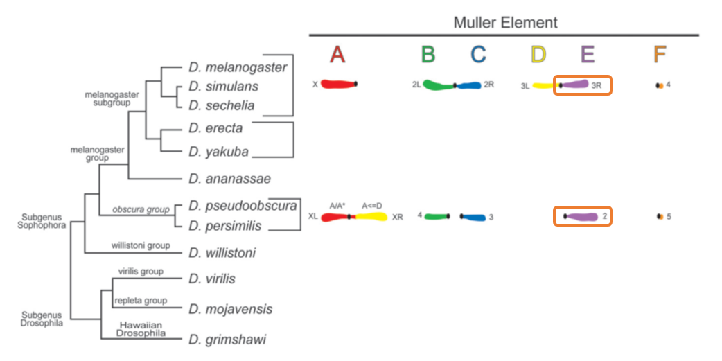
You can catch problems before you use the data in later analyses.Today we'll be talking about genome assembly. While the programs that perform the various steps of assembly have greatly improved over the past few years, genome assembly is still generally a slow, multi-step process. Given that, we'll be working with a smaller 150Mb genome from Drosophila pseudoobscura. Many times we will limit our data to just chromosome 2 (32Mb) of D. pseudoobscura to speed up run times even more.
D. pseudoobscura is a species of fruit fly that diverged from the well known D. melanogaster model species roughly 50 million years ago. D. pseudoobscura chromosome 2 is homologous to D. melanogaster chromosome arm 3R.
Using these data, we'll be performing the following tasks today:
- Assembling the D. pseudoobscura genome and assessing the quality of said assembly.
- Mapping reads from D. pseudoobscura chromosome 2 to D. melanogaster chromosome 3R.
- Assessing how iterative mapping of reads from D. pseudoobscura chromosome 2 to D. melanogaster affects divergence estimates.
Copying input data
The data we'll be working with today are mainly sequences in FASTA and FASTQ format (more on those in a moment). The input files are located on the server at
~/instructor_materials/Gregg_Thomas/congen-assembly/. Let's make a copy of this directory in our home directory so we don't
have to worry about that path anymore. First, make sure you are in your home directory:
cd ~| Command line parameter | Description |
|---|---|
| cd | The Linux change directory command |
| ~ | The path to the directory you want to change to. In bash,
~ is a shortcut meaning "the current user's home directory." |
Now let's make a copy of the data directory:
cp -r instructor_materials/Gregg_Thomas/congen-assembly/ .| Command line parameter | Description |
|---|---|
| cp | The Linux copy command |
| -r | Recursively copy all files in a directory. |
| instructor_materials/Gregg_Thomas/congen-assembly/ | The path to the directory you want to copy. |
| . | The path to the new copy. In bash, . is a shortcut meaning
"the same name." So this will copy the directory to our current location with the name congen-assembly |
Let's move into this folder with cd again since we'll spend the rest of the workshop here:
cd congen-assembly| Command line parameter | Description |
|---|---|
| cd | The Linux change directory command |
| congen-assembly | The path to the directory you want to change to. |
And now we can look at what is in that folder with the ls command. Make sure you've
selected your Terminal window and type the following:
ls| Command line parameter | Description |
|---|---|
| ls | The Linux list directory command to view the files in a folder. Shows files in current folder by default. |
You should see the following folders listed
| Folder | Description |
|---|---|
dmel-3R-reference/ | A folder containing the D. melanogaster chromosome 3R sequence file and its indices. |
dpse-chr2-reads/ | A folder containing Illumina short reads for D. pseudoobscura. |
expected-outputs/ | Pre-run outputs for all the programs we run today. If you get stuck or something takes too long, look for the expected output here |
scripts/ | A few supplementary scripts for data analysis. |
We have tried to anticipate the expected outputs from the commands we run today. If you get behind or stuck on something, try moving on to the next
step by adding expected-outputs/ to the beginning of the path for input you were expected to generate for the next command.
Feel free to ask us for help for any specific command.
Preparing output directories
I like to try and think ahead about what outputs my project will produce and make those directories early on, which helps me plan out my workflows. Today we'll be generating assemblies, read mappings, and alignments, so let's prepare an output directory for each of those tasks.
mkdir alignments| Command line parameter | Description |
|---|---|
| mkdir | The Linux make directory command |
| alignments | The name of the directory where we will generate and store our alignments for comparing assemblies and read mappings |
mkdir assemblies| Command line parameter | Description |
|---|---|
| mkdir | The Linux make directory command |
| assemblies | The name of the directory where we will generate and store our assemblies |
mkdir mapped-reads| Command line parameter | Description |
|---|---|
| mkdir | The Linux make directory command |
| mapped-reads | The name of the directory where we will generate and store our read mappings |
We'll also be running the program FastQC, which requires a pre-made output directory:
mkdir fastqc-output| Command line parameter | Description |
|---|---|
| mkdir | The Linux make directory command |
| fastqc-output | The desired name of the new directory. |
Some other programs we run will create their own output directories. We should now be ready to run the commands to generate assemblies and read mappings. But first, let's get familiar with our input data, sequences and reads...